'data.frame': 2907 obs. of 9 variables:
$ country : Factor w/ 185 levels "Albania","Algeria",..: 2 3 18 22 26 27 29 31 32 33 ...
$ year : int 1960 1960 1960 1960 1960 1960 1960 1960 1960 1960 ...
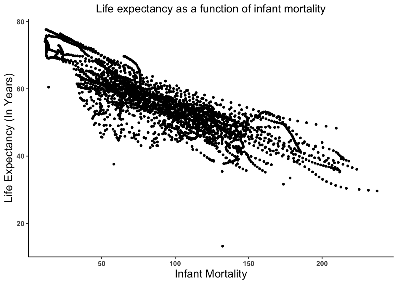
$ infant_mortality: num 148 208 187 116 161 ...
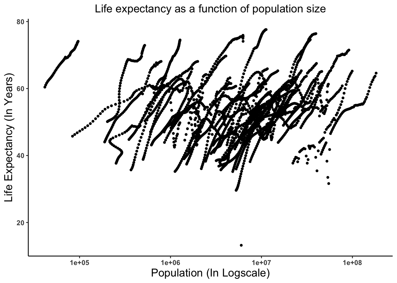
$ life_expectancy : num 47.5 36 38.3 50.3 35.2 ...
$ fertility : num 7.65 7.32 6.28 6.62 6.29 6.95 5.65 6.89 5.84 6.25 ...
$ population : num 11124892 5270844 2431620 524029 4829291 ...
$ gdp : num 1.38e+10 NA 6.22e+08 1.24e+08 5.97e+08 ...
$ continent : Factor w/ 5 levels "Africa","Americas",..: 1 1 1 1 1 1 1 1 1 1 ...
$ region : Factor w/ 22 levels "Australia and New Zealand",..: 11 10 20 17 20 5 10 20 10 10 ...
Rows: 2,907
Columns: 9
$ country          <fct> "Algeria", "Angola", "Benin", "Botswana", "Burkina Fa…
$ year             <int> 1960, 1960, 1960, 1960, 1960, 1960, 1960, 1960, 1960,…
$ infant_mortality <dbl> 148.2, 208.0, 186.9, 115.5, 161.3, 145.1, 166.9, NA, …
$ life_expectancy  <dbl> 47.50, 35.98, 38.29, 50.34, 35.21, 40.58, 43.46, 50.1…
$ fertility        <dbl> 7.65, 7.32, 6.28, 6.62, 6.29, 6.95, 5.65, 6.89, 5.84,…
$ population       <dbl> 11124892, 5270844, 2431620, 524029, 4829291, 2786740,…
$ gdp              <dbl> 13828152297, NA, 621797131, 124460933, 596612183, 341…
$ continent        <fct> Africa, Africa, Africa, Africa, Africa, Africa, Afric…
$ region           <fct> Northern Africa, Middle Africa, Western Africa, South…